What is an RL problem?

In recent years, we saw tremendous progress in Reinforcement Learning (RL). We saw that RL can be used to play Atari games (Minh et al.) by looking at the images of the game like we human do. RL is also used to master the Game of Go (Silver et al.). So an obvious question comes is what is RL and how is it used to solve such complicated problems?

In a nutshell, in a RL problem, there is an agent. It interacts with an environment. The environment presents a situation to the agent that we call state. The agent takes an action, the environment gives her a reward, and the environment presents a new state to the agent. This process goes on until some stopping criterion is met. The goal of the agent is to take actions that maximizes her total reward. The following figure summarizes what is an RL problem:

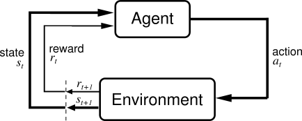
Notations used in the above figure:

1. State ($s_t$): State of the environment at time $t$
2. Action ($a_t$): The action taken by the agent at time $t$
3. Reward ($r_t$): The reward recieved by the agent at time $t$ for taking actions $a_t$ at state $s_t$
4. Trajectory: All the (states, actions, and rewards) tuple starting from time $0$ till some stopping criterion is met. $\left\{(s_0, a_0, r_0), (s_1, a_1, r_1), \cdots, (s_{T-1}, a_{T-1}, r_{T-1}), s_T)\right\}$.
5. Goal: Maximize the total reward ($r_0 + r_1 + \cdots + r_{T - 1}$)

There are mainly two type of approaches that are used to solve an RL problem.

1. Value Based (Critic Only)
2. Policy Based (Actor Only)

In the value based approaches, the agent keeps track of an estimate of goodness of an action at a given state. This estimate is called action-values and is usually denoted by $Q(s, a)$ where $s$ is the state and $a$ is the action. She takes action based on the estimate and receives a reward. She updates her estimate. Usually, after updating her estimates for sufficiently many times, she is able to find an appropriate measure of goodness of an action at a given state.

Note that the value based approaches are also known as critic only approaches because they only estimate an critic that tells the goodness of an action at a given state. The action is chosen based on this estimate.

Q-learning

One classical way to update action-values is Q-Learning. In Q-Learning, the agent updates its action-value estimate using the following equations: \begin{equation} Q(s, a) \leftarrow (1 - \alpha) \;Q(s, a) + \alpha \left(r + \gamma \max_{b} Q(s’, b)\right) \end{equation} where

• $s' \rightarrow$ next states,
• $r \rightarrow$ reward for taking action $a$ at state $s$
• $\alpha \rightarrow$ learning rate
• $\gamma \rightarrow$ discount factor

Q-Learning has been proven successful in learning a lot of challenging tasks. Playing Atari games from pixel is one of them. However, Q-learning has its own limitations. Q-learning is suspectible to numerical errors. It is difficult to incorporate continuous actions in Q-learning.

Policy-based approaches can solve some of the above problems of Q-learning. Policy is simply a mapping from the state to the action. Policy-based approaches are natural to incorporate continuous action spaces. Policy based approaches chanages the policy slowly towards an optimial policy so they are more stable in learning.

Note that the policy based approaches are also known as actor only approaches because they directly train an actor that tells what action to take at a given state. In contrast, value based approaches train a critic and actions are infered using the critic.

In the policy based approaches, the agent chooses a paramterized policy $\pi_\theta$. The agent takes actions according to this policy and receives the reward. She computes an estimate of the gradient of policy’s parameters with respect to the total reward and changes the parameters in the direction of gradient. One of the most basic policy-based algorithm is Vanila Policy Gradient.

Vanila Policy Gradient

Policy Gradient Algorithm starts with a randomly initialized (poor) policy. It then collects trajectories from this policy. It then changes the parameters of the policy so that it can make it a little better. It iterates over this process to find an optimal policy. In all of these processes, the most important part is the way we update a policy.

The way we improve the policy is based on the Policy Gradient Theorem (PGT). PGT says that if our objective is to find a policy that maximizes the total expected reward during an episode, then we should change the parameters of the policy in the following directions:

$$\Delta \theta = \mathbb{E}_{\{s_t, a_t\}_{t=0}^{T-1}} \left[\sum_{t = 1} ^ {T - 1} \left(\nabla_\theta\log \pi_\theta(a_t | s_t)\right) Q^{\pi_\theta}(s_t, a_t)\right]$$

Note that in the above equation we need to estimate action-value function $Q^{\pi_\theta}(s, a)$. There are many ways we can estimate action-value functions. One traditional way is to use Monte-Carlo Estimate in which we collect a lot of trajectories and use the cumulative rewards to estimate action-values. Although simple, the Monte-Carlo estimate suffers from high variance. To overcome the problem of high variance, the actor-critics algorithms are proposed.

Actor-Critic

In actor-critic algorithm alongwith learning the policy, we also learn the action-values. These actor-critic algorithms are the focus of this presentation where we will use a function-approximator to approximate action-values.

To estimate the action-values $Q^{\pi_\theta}(s, a)$ we modified the approach used in the DQN paper. Mainly, we estimate $Q^{\pi_\theta}(s, a)$ using the following equation:

\begin{equation} Q(s, a) \leftarrow (1 - \alpha) \;Q(s, a) + \alpha \left(r + \gamma \sum_{b} \pi_{\theta}(s, b) Q(s’, b)\right) \end{equation}

Note that the above equation is similar as in the Q-learning update except that instead of using the max action-values, we are using the averaged action-values. The rationale for using the above update is that this update converges to the action-values of the present policy while the previous update (Q-learning update) converges to the action-values of the optimal policy. We need the action-values of the present policies for policy gradient updates that is why we used the above updates.

Implementing the Actor-Critic Algorithm

We see that Actor-Critic algorithm utilizes the best of both policy-based and value-based algorithm. We decided to implement actor-critic algorithm for this presentation.

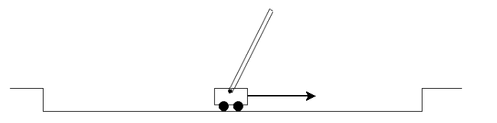
To solve a reinforcement learning problem, we choose a classical control problem called “Cartpole”. The cartpole problem is described in the openai gym documentation as following:

A pole is attached by an un-actuated joint to a cart, which moves along a frictionless track. The system is controlled by applying a force of $+1$ or $-1$ to the cart. The pendulum starts upright, and the goal is to prevent it from falling over. A reward of $+1$ is provided for every timestep that the pole remains upright. The episode ends when the pole is more than 15 degrees from vertical, or the cart moves more than $2.4$ units from the center.

Goal: We set our time horizon to $200$ time steps. In our experience, we found out that $200$ is a sufficiently big number to ensure that we found a good policy to balnce the cartpole for ever. Our goal is to create an agent that can keep the Cartpole stable for the $200$ time-steps using the actor-critic algoirthm. The maximum reward that we can obtained in this environment is $200$.

An Actor-Critic algorithm has two main components:

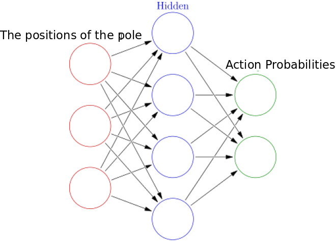
Policy Network ($\pi_\theta(s, a)$): The policy network tells us what actions to take by observing the position of the carpole. For example, in the following figure, we would hope that our learned policy network tell us that we should move our cart to right to balance the pole.

We use a neural network to represent the policy. The input to this neural network is the position of the pole and output is the probability of taking actions right or left as shown in the figure below.

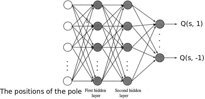
Value Network ($Q_w(s, a)$): The value network gives the estimated actions values that we use in the policy gradient theorem. We used a two hidden layer neural network to model a value network. The input to the value network is the positions of pole and the output is the action-values of the policy $\pi_\theta(s, a)$.

Work Flow

1. Initialize policy parameters ($\theta$) and value function parameters ($w$) arbitrary
2. do N times
   1. Collect a trajectory from the environment $(s_0, a_0, r_0, s_1, a_1, r_1, \cdots s_T, a_T, r_T)$ using policy $\pi_\theta$.
   2. Compute $Q_w(s, a)$ for all state and action pairs seen in the trajecory.
   3. Update $\theta$ using the polcicy gradient theorem.
   4. Update $w$ to minimize the loss \begin{equation} \min_w \left(Q_w(s, a) - \left(r + \gamma \sum_b \pi_\theta(s, b)Q_w(s, b)\right)\right)^2 \end{equation}

An epic failure

The first time, we implemented and run our actor-critic algorithm, we saw an epic failure. One of the example of this epic failure is in the following image.

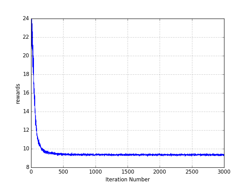
It does not matter how much hyper-parameter tuning we did, our total reward per episode was not going up at all. We explored further and we found out that the policy that our algorithm has learnt was a deterministic policy such that it always took the same action at all the states. Clearly, a policy that tells the agent to take the same action at all the states cannot be optimal for a cartpole environment. The proposed Actor-Critic algorithm was always converging to this deterministic policy independent of whatever initial weights we chose. This puzzled us.

A mathematical explanation of the epic failure

During our hunt in finding the reason behind the failure, we came across a shocking observation: all deterministic policies are the local minima in the Vanilla Policy Gradient algorithm.

To explore it further, note that the update in the VPG is

$$\Delta \theta = \mathbb{E}_{\{s_t, a_t\}_{t=0}^{T-1}}\left[\sum_{t = 0} ^ {T - 1} \left(\nabla_\theta\log \pi_\theta(a_t | s_t)\right) Q^{\pi_\theta}(s_t, a_t)\right]$$

We will show that whenever $\pi_\theta$ is a deterministic policy, then $\Delta \theta = 0$.

Proof: We use a neural network to generate the logit for the policy $\pi_\theta$. We then use a softmax layer to produce the probability. Since $\pi_\theta$ is a deterministic policy, it always generate one unique action at a given state. Using the calculus, the derivative of the loss with respect to the $l^{th}$ logit will be $\mathbb{E}_{\{s_t, a_t\}_{t=0}^{T-1}}\left[\left(\mathbb{1}(l|s_i) - \pi_\theta(l| s_i)\right)Q^{\pi_\theta}(s_t, a_t)\right]$ where $\mathbb{1}(l|s_i)$ is an identity function such that $\mathbb{1}(l|s_i) = 1$ when $l = a_i$ otherwise $0$. Since $\pi_\theta$ is a deterministic policy, $\pi_\theta(l|s_i) = 1$ only when $l = a_i$ otherwise $0$. Hence the derivative of the logit with respect to the loss will be zero. Consequently, the derivative of all parameters in the neural network will have $0$ derivative with respect to loss becasue of the backpropogation algorithm.

Conclusion: Our proposed algorithm was finding a deterministic policy that always took the same actions at all the states and sticking to it since no gradient information was coming to tell it that this is not an optimal policy.

A solution (introducing the entropy)

Since we do not want our learnt policy to converge to the deterministic policy that take the same actions at all the states, we decided to change our reward function such that no deterministic policy is the local optimum of this reward function. The additional reward that we add is the entropy of the policy.

What is entropy?

In information-theoretic terms, entropy is a measure of the uncertainty in a system.

Consider a probability mass function (PMF) $\pi$ with probability masses $p_1,p_2,\ldots{},p_n$ (say), with $\sum_{i=1}^np_i=1$.

Mathematically, its entropy $H(\pi)$ is defined as $H(\pi)=-\sum_{i=1}^np_i\log_2 p_i$ bits.

For illustration, we use the example of tossing a unfair coin, where the probability of landing heads or tails is not necessarily $1/2$. The toss outcome may be modeled as a Bernoulli PMF with only two masses: $p_H=p$ and $p_T=(1-p)$, where $p_H$ and $p_T$ are the probabilities of obtaining a head or a tail respectively. The entropy of the coin toss experiment is $H(p)=-p\log_2 p -(1-p)\log_2(1-p)$. The figure below plots H versus p.

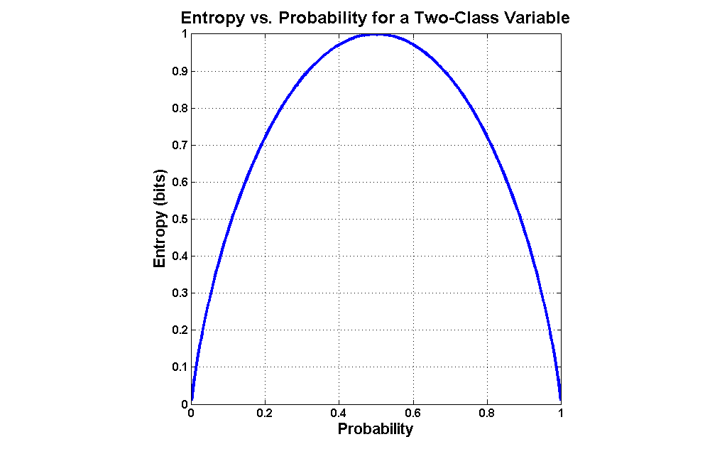
We see that the entropy is maximized when $p=0.5$, and minimized when $p=0$ or $p=1$. $p=1/2$ is the situation of maximum uncertainty when it’s most difficult to predict the toss outcome; the result of each coin toss delivers one bit of information. When the coin is not fair, the toss delivers less than one bit of information. The extreme case is that of a double-headed coin that never comes up tails, or a double-tailed coin that never results in a head. Then there is no uncertainty. The entropy is zero: each toss of the coin delivers no new information as the outcome of each coin toss is always certain.

The key idea to take from the above definition of entropy is that if we include an additional reward that is the entropy of the policy then we will favour a random policy in comparison to a fixed policies.

Based on this idea we modified our policy gradient reward as following:

Policy Gradient Reward: \begin{equation} \sum_t \left(r_t + 0.5 \text{Entropy}\left(\pi(.|s_t,\theta\right)\right) \end{equation} We change $\theta$ parameters in the direction such that we maximize the above defined reward. Note that the reason for choosing the constant $0.5$ for multiplying factor for entropy is empirical.

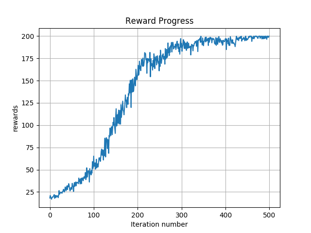
Result

After modifying the policy gradient reward, we ran the Vanilla Policy Gradient algorithm and you can see the result of one run in the following figure:

Concluding remarks

From this presentation, we note that adding an entropy bonus when solving an RL problem using the actor-critic approach can be crucial. It helps in the policy not sticking to a sub-optimal deterministic policy.

References:

1. A good introduction to Policy Gradient Algorithm: Karpathy’s RL Blog
2. Nervana blog
3. An state of the art actor-critic approach using entropy bonus