Can you identify a user from their bash history?
Using deep learning to identify unique user patterns
Preface: This was a small side scenario that came out of of a research project in the AI group at Samsung SDS Research America.
The question seems pretty reasonable, your average shell user probably spends some amount of time in their home directory, reading and writing files with unique names.
# Start Session 1
cd ~/private/docs
ls -laF | more
cat foo.txt bar.txt zorch.txt > somewhere
exit
# End Session 1
Given enough sessions you could probably learn a simple filename=>user dictionary with reasonable accuracy to predict the users identity.
but what if your bash history looks like this
**SOF**
cd
<1>			# one "file name" argument
ls
-laF
|
more
cat
<3>			# three "file" arguments
>
<1>
exit
**EOF**
Obtained from the UNIX User Data UC Irvine KDD Archive.
This log actually represent the same session as above, except “sanitized to remove filenames, user names, directory structures, web addresses, host names, and other possibly identifying items.”
This is where the story starts and things get interesting. Here we have a dataset explicitly sanitized to remove any personal identifying information, can we still identify the user simply from the pattern of their shell commands.
Each of us has our own unique expression that comes out in everything we do, it’s something that we can’t help but do. From the way we write to the way we walk and talk, we can recognize in people a certain quality that is often hard to describe but easy to identify. Our brains are incredibly good at tasks like these and one of the big directions in AI is teaching computers to think in this way. We can broadly refer to this as computer perception and it’s an area that deep learning has been particularly successful.
The command line is a very coarse interface, like a language with a very small vocabulary. Our hope is that even with such a small vocabulary we might be able to find something sufficiently unique quality about a user to identify them in the future. Of course, we aren’t doing this, our deep learning model will.
Note: There is an obvious privacy consideration here. Are we trying to deanonymize data that has been purposefully anonymized? Sort of, it sure looks like it at a glance. But we’re not recovering any personal information, we can’t. What we’re learning is whether this one anonymous person’s behavior patterns match another anonymous person’s behavior patterns. This is similar to handwriting identification. If you’re trying to match handwriting samples, you can’t tell who the samples belong to, but if you’re good enough at analyzing handwriting, you can tell you if they belong to the same person or not.
The Goal
We want to build and train a model to read in a sequence of shell commands and have it tell us which user most likely typed that sequence of commands. That is, the model is going to output a probability score over the class of known users.
what does the data look like?
This is the due diligence part of machine learning and data science work, and it’s always good to understand the dataset.
We’re using the UNIX User Data dataset from the UC Irvine KDD Archive.
The dataset is made up of shell sessions logs from 9 different users, all the logs are all already sanitized and labeled implicitly by the user they belong to. The raw data resembles the sanitized session shown above.
| User | # of sessions | avg session length | % of dataset |
|---|---|---|---|
| 0 | 562 | 16.0 | 6.2% |
| 1 | 488 | 40.6 | 5.4% |
| 2 | 755 | 24.0 | 8.3% |
| 3 | 484 | 34.5 | 5.3% |
| 4 | 911 | 41.4 | 10.0% |
| 5 | 546 | 63.6 | 6.0% |
| 6 | 2425 | 25.6 | 26.6% |
| 7 | 1339 | 12.7 | 14.7% |
| 8 | 1590 | 33.5 | 17.5% |
Ok, so our data is pretty skewed. That is, the sessions are not identically distributed across the labels (users). That is to be expected, and reflects the typical scenarios encountered in the real world. In principle, we could subsample the data so that it’s close to identically distributed but we’re going to leave it as is because 9100 samples is already not a lot to work with.
When working with skewed data, models that aren’t able to learn anything meaningful from the inputs will start to simply fit to the frequency of the labels. In our case, a bad model would associate every session to user 6, and it would be correct about 26.6% of the time, which is better than guessing uniformly randomly (11.1% accuracy).
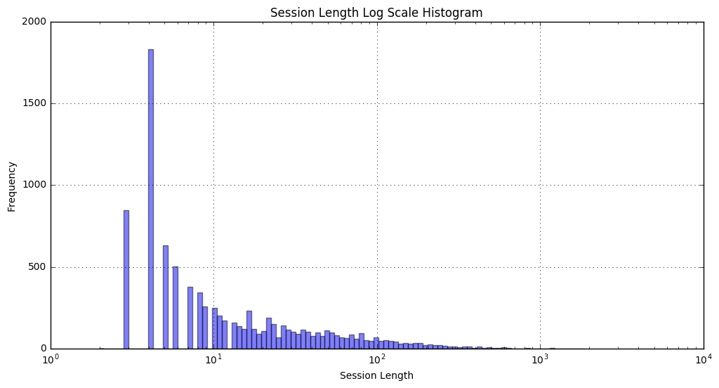
Additionally, as you can see in the histogram above, the distribution of session lengths is heavily skewed towards short sessions. Even with the log scale in the x-axis, we see an exponential decay in frequency of long sessions.
The session lengths are skewed similarly for each of the users individually as well.
Something to note is that the session length counts the **SOF** and **EOF** as commands, these are not commands input by the user but they are potentially relevant to the learning algorithm to know when a session starts and ends, so we keep them.
Here’s the first few bars of the histogram in tablular form.
| Session Length (user commands) | Frequency | % of dataset |
|---|---|---|
| 3 ( 1 ) | 848 | 9.3% |
| 4 ( 2 ) | 1830 | 20.1% |
| 5 ( 3 ) | 630 | 6.9% |
| 6 ( 4 ) | 504 | 5.5% |
| 7 ( 5 ) | 380 | 4.2% |
| 8 ( 6 ) | 342 | 3.8% |
| 9 ( 7 ) | 257 | 2.8% |
| >9 ( >7 ) | 4059 | 47.4% |
We haven’t even started doing any training, but we can expect that this will pose a bit of a challenge. How much accuracy can we reasonably expect when almost 10% of our sessions contain just one user command.
data pre-processing
Our inputs are sequences of strings (commands or arguments), we’re going to build a dictionary for the neural net to understand the sequences numerically
dic = {}
index = 1
for s in itertools.chain.from_iterable(sequences):
    if s not in dic:
        dic[s] = index
        index += 1
The actual numerical keys (integers) we assign to each command or argument are not important, only that they are distinct integers.
We’re not going to pad the entire data set, that would be extremely inefficient. Most of our sessions are very short, but some are over a thousand commands long, padding the whole dataset to max length would mean each forward pass would be processing thousands of null commands each iteration for no reason.
We’ll be using Tensorflow, Google’s open-source machine learning library. It allows the user to define a computational graph to be run with some desired input. The actual graph execution is handled by Tensorflow using whatever hardware is locally available. It has a great community of users and contributors providing cutting edge features, portability and scalability.
One of Tensorflow’s big strengths is allowing great flexibility in reading/batching/transforming the data inside the computational graph before it hits the actual model. The dynamic_pad option in the tf.train.batch class will allow the sequences in our bash history dataset to be variable length but will still pad them in batches (for batch processing) on the fly. Batch processing has the double benefit of speeding up computation as well as reducing the noise in calculating the optimization gradient.
We’ll also be processing the data into tf.train.Example objects (in our case tf.train.SequenceExample) and dumping these to TFRecords files. This makes the data pipeline much cleaner and faster in Tensorflow.
def make_example(sequence, labels):
    # The object we return
    ex = tf.train.SequenceExample()
    # A non-sequential feature of our example
    sequence_length = len(sequence)
    ex.context.feature["length"].int64_list.value.append(sequence_length)
    # Feature lists for the two sequential features of our example
    fl_tokens = ex.feature_lists.feature_list["tokens"]
    fl_labels = ex.feature_lists.feature_list["labels"]
    for token, label in zip(sequence, labels):
        fl_tokens.feature.add().int64_list.value.append(token)
        fl_labels.feature.add().int64_list.value.append(label)
    return ex
This creates a tf.train.SequenceExample object which can be serialized by calling ex.SerializeToString() and dumped to a TFRecords file with tf.python_io.TFRecordWriter.
Besides reading, splitting the raw data by session, and mapping strings to ints with the dictionary, there isn’t any other pre-processing to be done outside the computational graph.
A simple baseline
We can test our future models against our initial idea of using word/command frequency to guess the user. This is a bag-of-words model, it ignores all grammar completely and just counts how many times each word/command shows up in a session. Then, it fit this to the class of known users with some simple linear classifier.
Logistic regression ends up winning out as the best classifier for this dataset. We get the following baseline result.
Top-1 Train Accuracy: 71.2%
Top-1 Test Accuracy: 64.0%
Not terrible, but definitely leaves room for improvement.
The Model
In a very broad sense, we’re trying to classify sequential data and our baseline model ignores the sequential nature of the data completely. One challenge in working with this type of data is that the sequences are of variable length. If we have any hopes of deploying such a model, it needs to be able to handle sequences of arbitrary length. Our baseline model solved this by mapping each sequence to a fixed length vector of word frequencies.
If we’re thinking of using the sequential nature of the data and a deep learning architectures (and we are), this basically means we need a recurrent neural net.
Here is a great intro to recurrent neural networks
Here is high level diagram of what a rollout of the network looks like for a single sample.

This is a common base recurrent architecture for a sequence classifier.
- The input sequence (green) goes into the recurrent portion of the network one command at a time, the recurrent node (blue LSTM cell) returns an output (up arrow) and its internal state (right arrow) to itself for the next command.
- Mask (grey) the sequence of outputs from the recurrent node to collect just last one corresponding to input
**EOF**. Since the sequences are of variable length, the mask takes the length of the sequence as an input. - Feed the masked output through some number (2) fully connected layers (red) and a softmax layer to map down to the classification probability space.
- The output (yellow) is a
N_CLASSESdimensional probability vector. The user/class with the highest probability in that vector is the one the model believes to the (green) sequence originated from.
Some simple ways we can ramp this model up
- Larger layers: more parameters. We’re using LSTM (64) and FC1 (32), this could easily be expanded.
- Stacking recurrent layers and/or making the RNN rollout bidirectional
- More fully connected layers between the RNN portion and output
Other things to do
- Switch out the fixed mask for a learnable attention mechanism with an aggregating node
- Incorporate the final LSTM state output (the arrow pointing to the right from the LSTM cells, not shown for the final state output) into the prediction
Attention is a very interesting technique which allows the model to focus on certain inputs over others, but it counter-intuitively computationally expensive to do. It has proven very useful in natural language translation and in general can be a good introspection tool for ‘seeing’ what parts of the data the network is focusing on.
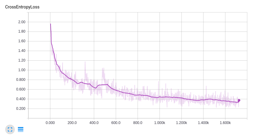
The Results
We trained with 80% of the data and reserved the remaining 20% for a validation test. Here are the tensorboard charts for the cross-entropy loss and top-1 training accuracy.
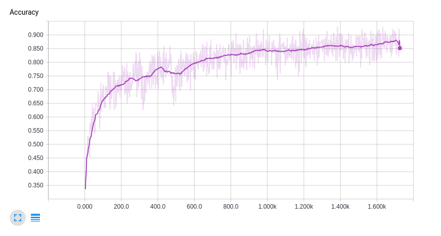
 Top-1 Train Accuracy: 88.0%
Top-1 Test Accuracy: 80.2%
This test accuracy is pretty good considering that 29.4% of the bash sessions are two commands or fewer, it’s somewhat surprised the model is able to do so well. We suspect we are benefiting from the small group of users and big dictionary size.
Also, the model is learning very quickly. This model can run on a laptop processing about one batch (128 samples)/sec, we’re looking at about 30 minutes of laptop training. If you eyeball the curve, it looks like we might eek out a percentage point or so if we train for a while longer.
With hundreds/thousands of users, the accuracy would drop pretty quickly unless we had substantially more data for each user or modified our approach.
Possible Security Application
The idea for this application is that in standard security protocols (disclaimer: not a security expert), a user is authenticated at start of session and trusted until end of session. This leaves open the problem of somebody taking over mid-session, either because they simply stepped away from the terminal or perhaps their credientials have been compromised.
What if we could verify user authenticity mid-session without any request to the user? If a user fails the verification then you ask them to re-authenticate in the standard way or stop their session. If you want to avoid kicking off legitimate users and/or annoying your customers, you need your accuracy to be pretty high or have a very high confidence intervals for your labeling.
What we’re talking about here is called active authentication or continuous authentication, it’s an active area of research and promises to solve some age old security problems like users walking away from their terminals without logging out.
The DARPA link is the #1 Google result for active authentication, this project is not affiliated with DARPA or their work on active authentication.
Final Thoughts
The results are pretty good given the amount of data we had available. We showed we could identify the user from their bash history 80.2% of the time when choosing between 9 different users compared to our baseline bag-of-words model which could only achieve 64.0% accuracy, a relative improvement of 45% on top-1 error.
We briefly explored the idea of using this as a security application, we would like to see accuracy near 99% for something like that, and we really would need to analyze the rate of false-positives, false-negatives, etc. From a practical standpoint, our current model (one model for all users) is unusable as adding additional users would require retraining an entirely new model, moreover the accuracy would be sure to plummet with a large number of users.
In a future post we’ll explore additional techniques to improve on this result and look into ways to scale such a model for our proposed security application.
Looking at other data sources, it’d be interesting to try something similar with more ‘raw’ data like raw keyboard/mouse I/O with time stamps or ‘touch’ data from a smartphone touchscreen.